Material Calibration – A Deep Dive
Knowing how to represent the materials in the structure is one of the hurdles of using Abaqus for sophisticated modeling.
It’s really easy to define a basic linear elastic material model. It’s a little trickier to define a nonlinear elastic material, like rubber or elastomer, but you may learn more about that topic by attending some of our excellent courses.
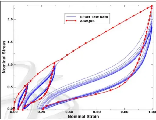
Rubber and elastomeric materials can get even more complicated than just their nonlinear elastic behavior, exhibiting significant viscous behavior and something called Mullin’s damage. The image above shows test data exhibiting all of these behaviors. It is very common that one needs to decide which behavior is important for your particular application. Trying to develop an “all-encompassing” material model that captures things such as rate dependence, temperature dependence, etc., is often not required to get some good design guidance from simulation.

We plan to write a number of articles that tackle typical problems with material modeling and calibration. We will be adding content to this article around every month, so please check back from time to time.
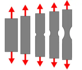
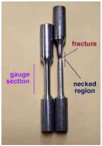
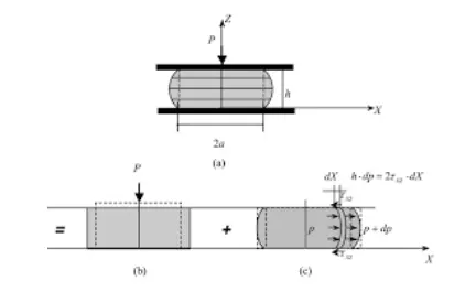
In the event that the measured portion of the specimen exhibits uniform material behavior, then calibration can be carried out using equations – if you know them. Two common non-homogeneous deformations are i) necking in a tensile test and ii) compression puck with friction. For non-homogeneous deformations, we often use multi-element Abaqus
analyses for calibration. Other times, the deformation might be homogeneous, but you don’t know the stress-strain relation equations (in closed form). In that case we often use Abaqus analysis of a “unit-cube” for calibration. We will have individual posts that describe each of these types of calibration approaches.
This Post will serve as an overview and summary of material test data that we can share with each other.


